
In the data analysis world, transforming raw data into meaningful insights often requires restructuring datasets to highlight patterns and relationships. Pandas, Python's premier data manipulation library, offers an exceptionally powerful tool for this purpose: the pivot table. Similar to pivot tables in spreadsheet applications but with greater flexibility and programmatic control, pandas pivot tables enable analysts to reshape, aggregate, and summarize data with remarkable ease. This article explores the functionality, techniques, and best practices for leveraging pivot tables in pandas to elevate your data analysis workflow.
Understanding Pandas Pivot Tables
At its core, a pivot table is a data summarization tool that rearranges and aggregates data from a tabular format into a more structured layout. The pandas implementation allows you to:
- Transform long/stacked data into a wide, matrix-like format
- Perform aggregations across multiple dimensions
- Create hierarchical indices for complex data relationships
- Apply different aggregation functions to various metrics
- Generate insights by highlighting relationships between variables
The Basic Pivot Table
The fundamental function for creating pivot tables in pandas is pivot_table(). Its basic syntax is:
pandas.pivot_table(data, values=None, index=None, columns=None, aggfunc='mean')
Let's break down the key parameters:
- data: The DataFrame containing your source data
- values: The column(s) you want to aggregate
- index: The column(s) to use as row labels
- columns: The column(s) to use as column labels
- aggfunc: The function(s) used to aggregate values (default is mean)
A Simple Example
Consider a dataset of sales records:
import pandas as pd
import numpy as np

# Create sample sales data
data = {
    'Date': pd.date_range('2023-01-01', periods=100),
    'Product': np.random.choice(['Laptop', 'Phone', 'Tablet', 'Monitor'], 100),
    'Region': np.random.choice(['North', 'South', 'East', 'West'], 100),
    'Sales': np.random.randint(100, 1500, 100),
    'Units': np.random.randint(1, 10, 100)
}

df = pd.DataFrame(data)
To create a basic pivot table showing average sales by product and region:
pivot = pd.pivot_table(df,
                      values='Sales',
                      index='Product',
                      columns='Region')
print(pivot)
This produces a table with products as rows, regions as columns, and average sales as values.
Advanced Pivot Table Techniques
Multiple Aggregation Functions
One of the most powerful aspects of pandas pivot tables is the ability to apply multiple aggregation functions simultaneously:
pivot_multi = pd.pivot_table(df,
                           values=['Sales', 'Units'],
                           index='Product',
                           columns='Region',
                           aggfunc={'Sales': 'sum', 'Units': 'mean'})
print(pivot_multi)
This creates a hierarchical column structure showing the sum of sales and average units sold for each product-region combination.
Hierarchical Indices
For more complex analyses, you can create hierarchical indices on both rows and columns:
# Extract month from date
df['Month'] = df['Date'].dt.month_name()

pivot_hierarchical = pd.pivot_table(df,
                                  values='Sales',
                                  index=['Product', 'Month'],
                                  columns='Region')
print(pivot_hierarchical)
This provides a nested view of sales data, first organized by product, then by month, across different regions.
Handling Missing Values
Pivot tables often encounter missing values when certain combinations don't exist in the source data. Pandas offers options to handle these gaps:
pivot_fill = pd.pivot_table(df,
                          values='Sales',
                          index='Product',
                          columns='Region',
                          fill_value=0)  # Replace NaN with 0
print(pivot_fill)
Custom Aggregation Functions
Beyond the standard aggregation functions, you can define custom aggregations:
def sales_range(x):
    return x.max() - x.min()

pivot_custom = pd.pivot_table(df,
                            values='Sales',
                            index='Product',
                            columns='Region',
                            aggfunc=[np.mean, np.sum, sales_range])
print(pivot_custom)
This table shows the mean, sum, and range of sales for each product-region combination.
Margins and Grand Totals
Adding summary rows and columns enhances pivot tables with overall statistics:
pivot_margins = pd.pivot_table(df,
                             values='Sales',
                             index='Product',
                             columns='Region',
                             aggfunc='sum',
                             margins=True,
                             margins_name='Total')
print(pivot_margins)
The margins=True parameter adds a "Total" row and column showing the sum across each dimension.
Pivot Table Visualization
Visualizing pandas pivot tables can transform numerical data into compelling insights:
import matplotlib.pyplot as plt
import seaborn as sns

# Create a pivot table for visualization
pivot_viz = pd.pivot_table(df,
                         values='Sales',
                         index='Product',
                         columns='Region',
                         aggfunc='mean')

# Create a heatmap
plt.figure(figsize=(10, 8))
sns.heatmap(pivot_viz, annot=True, cmap='YlGnBu', fmt='.0f')
plt.title('Average Sales by Product and Region')
plt.tight_layout()
plt.show()
This code generates a heatmap visualizing the pivot table, making patterns immediately apparent.
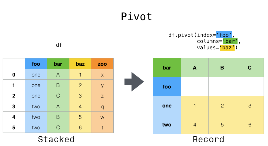
Pivot vs. Pivot_table
Pandas offers two similar functions: pivot() and pivot_table(). Understanding their differences is crucial:
- pivot(): Simple reshaping without aggregation. Requires unique index-column combinations.
- pivot_table(): More flexible, performs aggregation, and handles duplicate values.
Example of pivot():
# Simple pivot - will fail if duplicates exist
try:
    simple_pivot = df.pivot(index='Product', columns='Region', values='Sales')
    print(simple_pivot)
except ValueError as e:
    print(f"Error: {e}")
When your data contains duplicate combinations of index and columns, pivot() will raise an error, while pivot_table() will handle them by aggregating.
Real-World Applications
Financial Analysis
Pandas pivot tables excel at financial reporting, creating P&L statements, or analyzing financial metrics across different dimensions:
# Financial data example
finance_data = {
    'Date': pd.date_range('2023-01-01', periods=100),
    'Department': np.random.choice(['Marketing', 'Sales', 'R&D', 'Operations'], 100),
    'Category': np.random.choice(['Salary', 'Equipment', 'Software', 'Travel'], 100),
    'Expense': np.random.randint(1000, 10000, 100)
}

finance_df = pd.DataFrame(finance_data)
finance_df['Quarter'] = finance_df['Date'].dt.quarter

expense_report = pd.pivot_table(finance_df,
                               values='Expense',
                               index=['Department', 'Category'],
                               columns='Quarter',
                               aggfunc='sum',
                               margins=True)
print(expense_report)
Sales Analysis
Analyzing sales performance across products, regions, and time periods:
# Add a weekend/weekday flag
df['Day_Type'] = df['Date'].dt.dayofweek.apply(lambda x: 'Weekend' if x >= 5 else 'Weekday')

sales_analysis = pd.pivot_table(df,
                              values=['Sales', 'Units'],
                              index=['Product', 'Day_Type'],
                              columns='Region',
                              aggfunc={'Sales': 'sum', 'Units': 'sum'})
print(sales_analysis)
Marketing Campaign Analysis
Evaluating campaign performance across different segments:
# Marketing data example
marketing_data = {
    'Campaign': np.random.choice(['Email', 'Social', 'SEM', 'Display'], 100),
    'Segment': np.random.choice(['New', 'Returning', 'Lapsed'], 100),
    'Impressions': np.random.randint(1000, 10000, 100),
    'Clicks': np.random.randint(50, 500, 100),
    'Conversions': np.random.randint(1, 50, 100)
}

marketing_df = pd.DataFrame(marketing_data)
marketing_df['CTR'] = marketing_df['Clicks'] / marketing_df['Impressions']
marketing_df['CVR'] = marketing_df['Conversions'] / marketing_df['Clicks']

campaign_analysis = pd.pivot_table(marketing_df,
                                 values=['Impressions', 'Clicks', 'Conversions', 'CTR', 'CVR'],
                                 index='Campaign',
                                 columns='Segment',
                                 aggfunc={'Impressions': 'sum',
                                          'Clicks': 'sum',
                                          'Conversions': 'sum',
                                          'CTR': 'mean',
                                          'CVR': 'mean'})
print(campaign_analysis)
Performance Optimization
For large datasets, pandas pivot tables can become memory-intensive. Consider these optimization techniques:
Pre-aggregation
Aggregate your data before pivoting to reduce memory usage:
# Pre-aggregate before pivoting
pre_agg = df.groupby(['Product', 'Region']).agg({'Sales': 'sum', 'Units': 'mean'}).reset_index()
pivot_optimized = pd.pivot_table(pre_agg,
                               values=['Sales', 'Units'],
                               index='Product',
                               columns='Region')
print(pivot_optimized)
Filtering Data
Only include the necessary data points:
# Filter data before pivoting
filtered_df = df[df['Sales'] > 500]
pivot_filtered = pd.pivot_table(filtered_df,
                              values='Sales',
                              index='Product',
                              columns='Region')
print(pivot_filtered)
From Pivot Table to Original Data
Sometimes you need to convert a pandas pivot table back to a long format. The melt() function accomplishes this:
# Create a simple pivot table
simple_pivot = pd.pivot_table(df,
                            values='Sales',
                            index='Product',
                            columns='Region',
                            aggfunc='sum')

# Reset index to make 'Product' a regular column
simple_pivot_reset = simple_pivot.reset_index()

# Melt the pivot table back to long format
melted_pivot = pd.melt(simple_pivot_reset,
                      id_vars=['Product'],
                      value_name='Sales',
                      var_name='Region')
print(melted_pivot)
This process transforms the wide pivot table format back into a long dataframe, useful for further analysis or visualization.
Common Challenges and Solutions
Dealing with MultiIndex
Pivot tables often create MultiIndex structures, which can be challenging to work with:
# Create a pivot table with MultiIndex
multi_pivot = pd.pivot_table(df,
                           values=['Sales', 'Units'],
                           index=['Product', 'Month'],
                           columns='Region')

# Access specific values
value = multi_pivot.loc['Laptop', 'January']['Sales', 'North']
print(f"January Laptop Sales in North: {value}")

# Flatten a MultiIndex pivot table
flat_pivot = multi_pivot.stack().reset_index()
print(flat_pivot.head())
Conditional Formatting
To highlight important insights:
# Create a style object
styled_pivot = pivot_margins.style.highlight_max(color='lightgreen', axis=0)

# Add data bars for visual comparison
styled_pivot = styled_pivot.bar(subset=['Total'], color='#d65f5f')

# Format values as currency
styled_pivot = styled_pivot.format("${:.2f}")

# Display the styled pivot table
styled_pivot
Best Practices for Pandas Pivot Tables
- Start Simple: Begin with basic pivots before adding complexity.
- Handle Missing Values: Decide how to treat NaN values based on your analysis needs.
- Consider Readability: Use hierarchical indices judiciously; too many levels can reduce clarity.
- Optimize Performance: Filter and pre-aggregate data when working with large datasets.
- Document Aggregation Choices: Make explicit which aggregation functions are used for each metric.
- Combine with Visualization: Pivot tables paired with visualizations create powerful insights.
- Format Output: Apply styling to highlight important patterns and improve readability.
Pandas pivot tables stand as one of the most powerful tools in a data analyst's toolkit. By transforming raw data into structured, aggregated formats, they enable deeper insights and clearer communication of findings. Whether you're analyzing financial reports, marketing campaigns, sales performance, or any other multidimensional data, mastering pivot tables will significantly enhance your data analysis capabilities.